6. Intuitive Limits and Continuity
b. Intuitive Definitions
1. Left and Right Limits
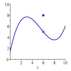
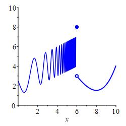
Given a function, \(f(x)\), and a point, \(x=a\), there are \(3\) quantities which describe the behavior of \(f(x)\) at and near \(x=a\).
The value of the function is \(f(a)\).
In the plot, \(a=6\) and \(f(6)=8\) which is the solid circle at \((6,8)\).
The limit of the function, \(f(x)\), as \(x\) approaches \(a\) from the left is the number, \(L\), that \(f(x)\) approaches as \(x\) approaches \(a\) from the left. We write: \[ \lim_{x\to a^-}f(x)=L \] In the plot, \(a=6\) and \(L=5\) which is the open circle at \((6,5)\).
The limit of the function, \(f(x)\), as \(x\)
approaches \(a\) from the right is the number, \(L\), that
\(f(x)\) approaches as \(x\) approaches \(a\) from the right. We write:
\[
\lim_{x\to a^+}f(x)=L
\]
In the plot, \(a=6\) and \(L=3\) which is the open circle at \((6,3)\).

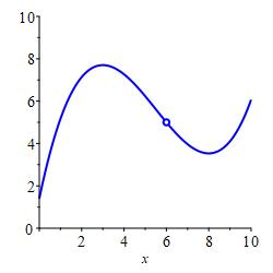
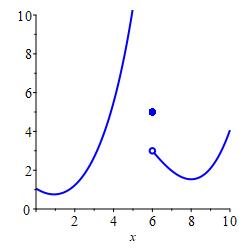
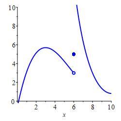
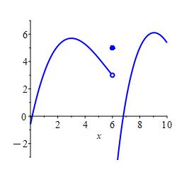
All three of these numbers may or may not exist and, in general, they can all be different. In the plot above, all three numbers exist and are all different. In the plot on the left below, the function value exists but is different from the limits from the left and right which happen to be equal. In the plot on the right below, the limits from the left and right exist and happen to be equal while the function value does not even exist. This has no effect on the limit. The limits are only concerned with what values \(f(x)\) approaches as \(x\) nears \(a\).
In this case, \(\displaystyle \lim_{x\to 6^-}f(x) =\lim_{x\to 6^+}f(x) =5\)
Again, \(\displaystyle \lim_{x\to 6^-}f(x) =\lim_{x\to 6^+}f(x) =5\)
If a limit exists, we say it converges.
If a limit does not exist, we say it diverges.
This is a intuitive preliminary definition. The actual precise definition appears on a later page. However, the precise definition is not essential for this course. Everything can be based on the intuitive definition.
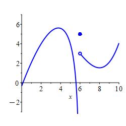
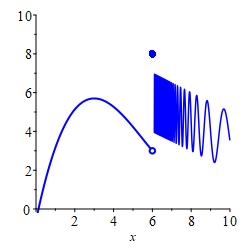
When Limits Do Not Exist
The six plots below show six situations in which a limit from the left or right does not exist.
from the left.
from the right.
We say a left or right limit is positive
infinity if \(f(x)\) gets arbitrarily large and positive
as \(x\) approaches \(a\) from the left or right (resp.).
We also say \(f(x)\) diverges to \(\infty\)
on the left or right and write:
\[
\lim_{x\to a^-}f(x)=\infty \qquad
\lim_{x\to a^+}f(x)=\infty \qquad \text{resp.}
\]
We say a left or right limit is negative infinity if \(f(x)\) gets arbitrarily large and negative as \(x\) approaches \(a\) from the left or right (resp.). We also say \(f(x)\) diverges to \(-\infty\) on the left or right and write: \[ \lim_{x\to a^-}f(x)=-\infty \qquad \lim_{x\to a^+}f(x)=-\infty \qquad \text{resp.} \]
We say a left or right limit is oscillitory divergent if the limit does not exist and is neither positive nor negative infinity.
To say a limit is defined to be \(\pm\infty\) does not say the limit exists, it merely says the way in which it diverges!
Click the refresh button to get a new plot.
For the function plotted, compute each quantity.
-
The limit from the left at .
Use the curve on the left of . The limit from the left is the height \(f(x)\) approaches as \(x\) approaches from the left, i.e. \(x\) is less than but getting very close to .
I can't understand your answer. It may have been typed wrong. I am expecting an integer, infinity, -infinity or undefined.
because the curve on the left goes to height as \(x\) goes to .
-
The limit from the right at .
Use the curve on the right of . The limit from the right is the height \(f(x)\) approaches as \(x\) approaches from the right, i.e. \(x\) is greater than but getting very close to .
Excellent! because the curve on the right goes to height as \(x\) goes to .
Sorry. Read the hint. Try again.
I can't understand your answer. It may have been typed wrong. I am expecting an integer, infinity, -infinity or undefined.
You need to enter an answer before checking.
because the curve on the right goes to height as \(x\) goes to .
-
The function value at . Enter a number or undefined.
is the value of \(f(x)\) at if it is defined. This is the solid dot above if there is one.
Good Job! because the solid dot above is at height .
Sorry. Read the hint. Try again.
I can't understand your answer. It may have been typed wrong. I am expecting an integer, infinity, -infinity or undefined.
You need to enter an answer before checking.
because the solid dot above is at height .
Click the refresh button to get a new piecewise function.
For the piecewise function shown, compute each quantity.
-
The limit from the left at .
The limit from the left is the value \(f(x)\) approaches if \(x \lt\) but getting closer to . So we successively plug , into the formula for \(x \lt\) . The limit is what we get by plugging \(x=\) into the formula for \(x \lt\) .
Perfect! because this is the result when one plugs into the formula for \(x \lt\) .
Sorry. Read the hint. Try again.
I can't understand your answer. It may have been typed wrong. I am expecting an integer, infinity, -infinity or undefined.
You need to enter an answer before checking.
because this is the result when one plugs into the formula for \(x \lt\) .
-
The limit from the right at .
.The limit from the right is the value \(f(x)\) approaches if \(x \gt\) but getting closer to . So we successively plug , into the formula for \(x \gt\) . The limit is what we get by plugging into the formula for \(x \gt\) .
Impressive! because this is the result when one plugs into the formula for \(x \gt\) .
Sorry. Read the hint. Try again.
I can't understand your answer. It may have been typed wrong. I am expecting an integer, infinity, -infinity or undefined.
You need to enter an answer before checking.
because this is the result when one plugs into the formula for \(x \gt\) .
-
The function value at . Enter a number or undefined.
The value of \(f(x)\) at is if it is defined. This is the value next to if there is one.
Good Job! because this is the value next to in the formula.
Way to go! is undefined because there is no value for .
Sorry. Read the hint. Try again.
I can't understand your answer. It may have been typed wrong. I am expecting an integer, infinity, -infinity or undefined.
You need to enter an answer before checking.
because this is the value next to in the formula.
Heading
Placeholder text: Lorem ipsum Lorem ipsum Lorem ipsum Lorem ipsum Lorem ipsum Lorem ipsum Lorem ipsum Lorem ipsum Lorem ipsum Lorem ipsum Lorem ipsum Lorem ipsum Lorem ipsum Lorem ipsum Lorem ipsum Lorem ipsum Lorem ipsum Lorem ipsum Lorem ipsum Lorem ipsum Lorem ipsum Lorem ipsum Lorem ipsum Lorem ipsum Lorem ipsum